3 Multiple Regression and Design Matrices

Exercise 1

For this exercise, we will consider the penguins data set from the palmerpenguins package (Horst, Hill, and Gorman 2020). The data set contains various measures of penguin size, species, and sex, along with the year and island when/where the observations were made. Begin by loading the data and dropping observations that have missing values for some of the predictors:

library(dplyr)
library(palmerpenguins)
data(penguins)
penguins <- penguins %>% filter(complete.cases(.))

First, consider a linear model in which you attempt to predict a penguin’s body mass (body_mass_g) from its flipper length (flipper_length_mm) and the sex (sex) of the penguin.

Fit the model using effects coding. Write down the entries in the design matrix, $X$ for the first 3 observations in the data set. Verify your answer using the model.matrix function. The first 3 observations are given by:

penguins[1:3,]

# A tibble: 3 × 8
  species island    bill_length_mm bill_depth_mm flipper_length_mm body_mass_g
  <fct>   <fct>              <dbl>         <dbl>             <int>       <int>
1 Adelie  Torgersen           39.1          18.7               181        3750
2 Adelie  Torgersen           39.5          17.4               186        3800
3 Adelie  Torgersen           40.3          18                 195        3250
# ℹ 2 more variables: sex <fct>, year <int>

Fit the same model using means coding. Again, write down the entries in the design matrix, $X$ for the first 3 observations in the data set. Verify your answer using the model.matrix function.
Now, consider adding species to the model in addition to flipper length (flipper_length-mm) and the sex (sex) of the penguin. Fit the model using effects coding. Write down the entries in the design matrix for the following observations:

penguins[c(1, 2, 200, 201, 300, 301),]

# A tibble: 6 × 8
  species   island    bill_length_mm bill_depth_mm flipper_length_mm body_mass_g
  <fct>     <fct>              <dbl>         <dbl>             <int>       <int>
1 Adelie    Torgersen           39.1          18.7               181        3750
2 Adelie    Torgersen           39.5          17.4               186        3800
3 Gentoo    Biscoe              46.5          14.4               217        4900
4 Gentoo    Biscoe              45            15.4               220        5050
5 Chinstrap Dream               49.7          18.6               195        3600
6 Chinstrap Dream               47.5          16.8               199        3900
# ℹ 2 more variables: sex <fct>, year <int>

Lastly, let’s allow the effect of flipper length to be sex-specific. This can be accomplished by adding an interaction between sex and flipper_length_mm, sex:flipper_length_mm to the model from [3] above. Again, write down the entries in the design matrix for 6 observations selected just above.

Exercise 2

For this exercise, we will use the leaftemp data set in the DAAG package (Maindonald and Braun 2020). The data set contains measurements of vapor pressure (vapPress) and differences between leaf and air temperatures (tempDiff) in an experiment conducted at three different levels of carbon dioxide (CO2level).

library(DAAG)
data(leaftemp)

Fit the following three models to these data:

simple linear regression: lm(tempDiff ~ vapPress, data = leaftemp)
Analysis of covariance: lm(tempDiff ~ vapPress + CO2level, data= leaftemp)
Interaction model: lm(tempDiff ~ vapPress*CO2level, data= leaftemp)

For the Analysis of covariance model, write down the equation for predicting the mean temperature difference as a function of vapor pressure for each of the 3 CO $_{2}$ levels.
For the Interaction model, write down the equation for predicting the mean temperature difference as a function of vapor pressure for each of the 3 CO $_{2}$ levels.
Plot the predicted mean temperature difference as a function of vapor pressure (and when appropriate, CO $_{2}$ level) for each of the 3 models.
Construct and fit a model in which each CO $_{2}$ level has a different intercept, but the medium and high CO $_{2}$ level treatments have the same slope for vapPress (which differs from the slope for the Low CO $_{2}$ level treatment).

Exercise 3

This example uses data from the Maryland Biological Stream Survey to explore added-variable and component+residual plots. To access the data, type:

library(Data4Ecologists)
data("longnosedace")

Predictors in the data set include:

stream: name of each sampled stream (i.e., the name associated with each case).
longnosedace: number of longnose dace (Rhinichthys cataractae) per 75-meter section of stream.
acreage: area (in acres) drained by the stream.
do2: the dissolved oxygen (in mg/liter).
maxdepth: the maximum depth (in cm) of the 75-meter segment of stream.
no3: nitrate concentration (mg/liter).
so4: sulfate concentration (mg/liter).
temp: the water temperature on the sampling date (in degrees C).

Begin by fitting a model containing all of the predictor variables in the data set (other than stream).
Create residual diagnostic plots to evaluate the assumptions of the linear regression model. Comment on whether or not you think each assumption of linear regression is met?
Explore the effect of each predictor (after accounting for all other predictors in the model) using added-variable plots constructed using the avPlots function in the car package. Just type avPlots(model-name) where model-name is the name you assign to the fitted model. When creating your report, you may want to adjust the size of the figure in the output using chunk options: fig.height = 12, fig.width=6, out.width = “80%”. You can also change the layout of the panels. For example, if you want a 2 x 3 set of panels (rather than the default 3 x 2), you can use avPlots(mod, layout = c(2, 3)).
Construct partial residual or component + residual plots using using the crPlots function in the car package via crPlots(model-name). Again, you may want to adjust the size of the plot and the layout of the panels.
Consider the added-variable and component + residual plots. Do these tell you anything more about potential assumption violations?
Component+residual plots can also be constructed using the termplot function (in base stats package) with the argument partial=T. The termplot function allows one to generalize the component+residual plot to more complicated models that allow for non-linear relationships¹. For example, we can construct a component+residual plot for a model with a quadratic term by replacing ${\hat{β}}_{i} X_{i}$ with ${\hat{β}}_{i 1} X_{i} + {\hat{β}}_{i 2} X_{i}^{2}$ . To see how the component + residual plot might look when non-linear terms are included in the model, consider a model with a quadratic effect of acreage and a linear effect of no3. I.e., mod2 <- lm(longnosedace ~ poly(acreage, 2) + no3, data=dace). Then produce a component + residual plot using: termplot(mod2, se=T, partial=T).

Exercise 4

Consider the data set birdmalariaLFS in the Data4Ecologists library. These data are associated with the following paper: Asghar, M., Hasselquist, D., Hansson, B., Zehtindjiev, P., Westerdahl, H., & Bensch, S. (2015). Hidden costs of infection: chronic malaria accelerates telomere degradation and senescence in wild birds. Science, 347(6220), 436-438.

The authors were interested in whether chronic infection might impact the fitness (e.g., number of offspring) of wild great reed warblers. The data set contains the following variables:

LFS = lifetime reproductive success (number of offspring produced)
Sex of bird (0 if male and 1 if female)
year = year of birth
Tlifespan = total lifespan (in years)
infected = infected status (0 = uninfected thoughout life, 1 = infected at 1 year of life and remained infected throughout life)
BTL = telomere length shortly after birth (telomere length is sometimes used to predict lifespan, but is not without controversy; see e.g., (Whittemore et al. 2019)).

The data set can be accessed using:

library(Data4Ecologists)
data("birdmalariaLFS")

The authors fit the following model relating Tlifespan to the other predictors:

mod1 <- lm(Tlifespan ~ Sex + year + BTL + infected + BTL:infected, data=birdmalariaLFS)
summary(mod1)


Call:
lm(formula = Tlifespan ~ Sex + year + BTL + infected + BTL:infected, 
    data = birdmalariaLFS)

Residuals:
    Min      1Q  Median      3Q     Max 
-2.2416 -0.8060 -0.2603  0.5255  5.2395 

Coefficients:
              Estimate Std. Error t value Pr(>|t|)    
(Intercept)  104.66665   87.76436   1.193 0.236791    
Sex           -0.36932    0.32120  -1.150 0.253869    
year          -0.05247    0.04411  -1.190 0.237980    
BTL            3.00839    0.78981   3.809 0.000283 ***
infected       2.60804    1.15466   2.259 0.026809 *  
BTL:infected  -3.86458    1.27743  -3.025 0.003401 ** 
---
Signif. codes:  0 '***' 0.001 '**' 0.01 '*' 0.05 '.' 0.1 ' ' 1

Residual standard error: 1.404 on 75 degrees of freedom
  (19 observations deleted due to missingness)
Multiple R-squared:  0.2408,    Adjusted R-squared:  0.1902 
F-statistic: 4.758 on 5 and 75 DF,  p-value: 0.0007873

Write down a set of equations for the model and interpret the model parameters in the context of the problem.
Write out the design matrix for the following 3 observations:

Observation 1: Sex = male, year = 1991, BTL = 0.80, infected = 1
Observation 2: Sex = female, year = 1991, BTL = 0.80, infected = 1
Observation 3: Sex = female, year = 1991, BTL = 0.80, infected = 0

Evaluate whether or not you think the assumptions of the linear regression model are met.

Exercise 5

The authors were interested in whether chronic infection might the impact fitness of wild great reed warblers. The data set contains the following variables:

LFS = lifetime reproductive success (number of offspring produced)
Sex of bird (0 if male? 1female)
year = year of birth
Tlifespan = total lifespan (in years)
infected = infected status (0 = uninfected thoughout life, 1 = infected at 1 year of life and remained infected throughout life)

The data set can be accessed using:

library(Data4Ecologists)
data("birdmalariaLFS")

Fit a linear model relating lifetime reproductive success to the sex of the bird, its birth year, total lifespan, and infected status. Allow the effect of total lifespan to differ for males and females. Also, assume the effect of birth year can be modeled using a continuous variable representing a trend over time.
Describe the model using a set of equations and interpret the model parameters in the context of the problem. Do not forget about $σ^{2}$ !
Write out the design matrix for the following 3 observations:

Observation 1: Sex = male, year = 1991, Tlifespan = 2, infected = 1
Observation 2: Sex = female, year = 1991, Tlifespan = 2, infected = 1
Observation 3: Sex = female, year = 1991, Tlifespan = 2, infected = 0

Exercise 6

This exercise was inspired by a contribution from Abigail Meyer. Abigail took FW8051 in the spring 2023.

For this exercise you will use data from (Koutrouditsou and Nudds 2021), originally stored on Dryad, and subsequently included in the Data4Ecologists package. The main objective of their study is nicely summarized in the abstract of their paper, which I’ve copied below:

The European swallowtail butterfly (Papilio machaon) is so named, because of the long and narrow prominences extending from the trailing edge of their hindwings and, although not a true tail, they are referred to as such. Despite being a defining feature, an unequivocal function for the tails is yet to be determined, with predator avoidance (diverting an attack from the rest of the body), and enhancement of aerodynamic performance suggested. The swallowtail, however, is sexually size dimorphic with females larger than males, but whether the tail is also sexually dimorphic is unknown. Here, museum specimens were used to determine whether sexual selection has played a role in the evolution of the swallowtail butterfly tails in a similar way to that seen in the tail streamers of the barn swallow (Hirundo rustica), where the males have longer streamers than those of the females.

You can access the data using:

library(Data4Ecologists)
data("Swallowtail")

Fit a linear regression model relating Tail_length to Sex and Hindwing_area using reference/effects coding.
1. Describe the model using equations.
2. Provide a clear interpretation of the regression coefficients.
Fit the same model using means coding.
1. Describe the model using equations.
2. Provide a clear interpretation of the regression coefficients.
Fit a a linear regression model relating Tail_length to Sex, Hindwing_area, and Species.
1. Describe the model using equations.
2. Provide a clear interpretation of the regression coefficients.
3. Write out the design matrix for the following two observations: 1) a male of species = Papilio machaon gorganus and with Hindwing_area = 4 cm $^{2}$ ; and 2) a female of species = Papilio machaon britannicus and with Hindwing_area = 3.6 cm $^{2}$ .
Since the above model has 2 categorical variables, it is not possible to re-express it using means coding for both of the categorical variables. If we subtract a 1, then R will use means coding for the first categorical variable that appears and effects coding for the second categorical variable. Verify this by fitting the following model: lm(Tail_length ~ Hindwing_area + Sex + Species -1, data = Swallowtail).
1. Describe the model using equations.
2. Provide a clear interpretation of the regression coefficients.
3. Write out the design matrix for the following two observations: 1) a male of species = Papilio machaon gorganus and with Hindwing_area = 4 cm $^{2}$ ; and 2) a female of species = Papilio machaon britannicus and with Hindwing_area = 3.6 cm $^{2}$ .

Exercise 7

This exercise is motivated by an exercise that was created by Conservation Sciences graduate student, Richard Hoover, who took this course in 2024.

Ontogeny, or the study of growth and development, is integral to understanding how organisms change over their lifespan. A key component to ontogeny is the concept of isometry. Isometry means that the relationship between traits – for example, head length to body length – should be proportional over time.² Thus, if we fit a linear model relating log(trait 1) to log(trait 2), the slope should equal 1. Deviations from isometry are referred to as allometry, which means unequal growth. A classic example of allometry is head size relative to body size in humans (toddlers have much larger heads in proportion to their body size than adults).

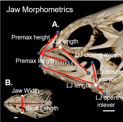
Richard studies prickleback fishes, which shift their diet as they age. In certain species, these fishes are carnivorous as juveniles but begin to incorporate algae into their diet with age, becoming omnivorous and then herbivorous. He is interested in how that relationship affects the feeding morphology of fish teeth and jaws.

Richard contributed the fishmorph data set in the Data4Ecologists package. These data can be read in using:

library(Data4Ecologists)
data(fishmorph)

To see a description of the data set and the variables it contains, you can access the help page by typing: ?fishmorph. Richard also shared a nice photo capturing the different measurements below:

For this exercise, we will focus on just 3 of the species:

AP = Anoplarchus purpurescens
PL = Pholis laeta
XA = Xiphister atropurpureus

We can select these species using the code below. I also recommend setting the options for page width using options, which will allow the ouptput of the regression models you fit to better fit within the page.

options(width = 120)
fishmorph2 <- subset(fishmorph, Species %in% c("Anoplarchus_purpurescens", 
                                               "Pholis_laeta",
                                               "Xiphister_atropurpureus"))

We will fit linear models relating logged values of lower jaw length (log(lj_length)) to logged values of skull length (log(skull_length)), allowing each species to have its own intercept and its own slope.

Begin by fitting the model using reference coding: lm(log(lj_length) ~ Species*log(skull_length), data = fishmorph2). Inspect the model using the summary function.
Describe the model using a set of equations and interpret the model parameters in the context of the problem. Do not forget about $σ^{2}$ ! To make life easier, feel free to abbreviate species names (using AP, PL, XA). Also, feel free to write the equations on a piece of paper, take a picture, and then include your picture using knitr::include_graphics (see ?knitr::include_graphics for help with this function). Or, write the equations using LaTex equivalent code using dollar signs to signify the start and end of equations. If you use LaTex, you may need to split the equation over multiple lines to prevent the equation from going off the page (if writing to pdf). Also, note that you may want to drop “_” from the variable names and use CammelCase (e.g., SkullLength) when writing equations using LaTex.
Write out the design matrix for the following 2 observations:

Observation 1: Species = Anoplarchus_purpurescens, log(skull__length) = 2
Observation 2: Species = Xiphister_atropurpureus, log(skull__length) = 1.5

Fit the same model using means coding. Write out the design matrix for the same two observations (above).
Using this model and the confint function, determine whether there is evidence for allometry (slope different from 1) for each of the 3 species.
Create a scatterplot of log(lj_length) versus log(skull_length) and overlay the fitted regression lines for each species.
The slopes for Species = Anoplarchus purpurescens and Species = Pholis laeta are nearly identical. Fit a model where the coefficient for log(skull_length) is the same for these two species, but where Xiphister atropurpureus has a different slope. Allow all 3 species to have their own intercept.
Plot predictions from the above model.

References

Horst, Allison Marie, Alison Presmanes Hill, and Kristen B Gorman. 2020. Palmerpenguins: Palmer Archipelago (Antarctica) Penguin Data. https://allisonhorst.github.io/palmerpenguins/.

Koutrouditsou, Lydia K, and Robert L Nudds. 2021. “No Evidence of Sexual Dimorphism in the Tails of the Swallowtail Butterflies Papilio Machaon Gorganus and p. M. Britannicus.” Ecology and Evolution 11 (9): 4744–49.

Maindonald, John H., and W. John Braun. 2020. DAAG: Data Analysis and Graphics Data and Functions. https://CRAN.R-project.org/package=DAAG.

Whittemore, Kurt, Elsa Vera, Eva Martı́nez-Nevado, Carola Sanpera, and Maria A Blasco. 2019. “Telomere Shortening Rate Predicts Species Life Span.” Proceedings of the National Academy of Sciences 116 (30): 15122–27.

Models cannot, however, include interaction terms.↩︎
When exploring relationships between traits, it is important to consider their dimensions. A length has 1 dimension, an area has 2 dimensions, and a volume or mass has 3 dimensions. If traits are isometric, then the slope relating the two traits should equal the ratio of their dimensions.↩︎