Chapter 16 Final Exam 2023

16.1 Exercise 1

Consider the data set birdmalariaLFS in the Data4Ecologists library. These data are associated with the following paper: Asghar, M., Hasselquist, D., Hansson, B., Zehtindjiev, P., Westerdahl, H., & Bensch, S. (2015). Hidden costs of infection: chronic malaria accelerates telomere degradation and senescence in wild birds. Science, 347(6220), 436-438.

The authors were interested in whether chronic infection might the impact fitness of wild great reed warblers. The data set contains the following variables:

LFS = lifetime reproductive success (number of offspring produced)
Sex of bird (0 if male? 1female)
year = year of birth
Tlifespan = total lifespan (in years)
infected = infected status (0 = uninfected thoughout life, 1 = infected at 1 year of life and remained infected throughout life)

The data set can be accessed using:

library(Data4Ecologists)
data("birdmalariaLFS")

Fit a linear model relating lifetime reproductive success to the sex of the bird, its birth year, total lifespan, and infected status. Allow the effect of total lifespan to differ for males and females. Also, assume the effect of birth year can be modeled using a continuous variable representing a trend over time. (2 pts)
Describe the model using a set of equations and interpret the model parameters in the context of the problem. Do not forget about \(\sigma^2\)! (7 pts)
Write out the design matrix for the following 3 observations: (2 pts)

Observation 1: Sex = male, year = 1991, Tlifespan = 2, infected = 1
Observation 2: Sex = female, year = 1991, Tlifespan = 2, infected = 1
Observation 3: Sex = female, year = 1991, Tlifespan = 2, infected = 0

Evaluate whether or not you think the assumptions of linear regression are met. Justify your answers by referring to characteristics in appropriate diagnostic plots. (4 pts)
Consider the characteristics of the response variable (LFS). Fit an alternative model to these data, but including the same set of predictor variables. Write down a set of equations describing the model and identify the parameter estimates in the output from R. (6 pts)
Use your model from step 5 to estimate the mean lifetime reproductive success for a female, born in 1991, that lives 5 years while infected with malaria. (3 pts)

16.2 Exercise 2

Harder and Thompson (1989)¹⁰ quantified the amount of pollen removed by bumblebee queens and honeybee workers as a function of the time they spent at flowers. These data can be accessed using:

library(Data4Ecologists)
data(beepollen)

The data set has three variables:

removed = proportion of the pollen removed
duration = duration of visit (in seconds)
queen = 1 if the been was a queen bee and 0 otherwise

Fit a linear model relating the amount of pollen removed from the plant (removed) as a function of the time spent at the flower (duration) and the type of bee (note queen = 1 if the bee is a queen bee or 0 if it is a worker bee). Evaluate the assumptions of the linear model. (4 pts)
Update the model to allow for a non-linear relationship between duration and removed. Again, check the assumptions of the model. (6 pts)
Create a plot of the data, overlaying the estimated mean response curve from step 2 separately for queen and non-queen bees (i.e., plot \(E[removed | duration, queen]\) and \(E[removed | duration, not queen]\) versus \(duration\)). For full credit, add confidence intervals for the mean response curve. (3 pts)
Use optim or JAGS to fit the following model: (5 pts)

\[\begin{gather} removed_i \sim N(\mu_i, \sigma^2)\\ \mu_i = (\beta_1 + \beta_2I(queen=1)_i)*\left(1 - exp(-\beta_3*duration_i)\right) \end{gather}\]

Note: the mean response pattern will asymptote at either \(\beta_1\) (for worker bees) or \(\beta_1 + \beta_2\) (for queen bees). The parameter \(\beta_3\) will control how fast the curve approaches the asymptote. If you use optim, you will need good starting values. You should be able to guess at the asympotote by plotting the data. For \(\beta_3\), a value around 0.07 should work well. If you fit the model using JAGS, you will need to specify priors. One option would be to specify priors for log(\(\beta_1\)) and log(\(\beta_3\)) so that \(\beta_1\) and \(\beta_3\) are ensured to be positive.

Create a plot of the data, overlaying the estimated mean response curve from step 4 separately for queen and non-queen bees (i.e., plot \(E[removed | duration, queen]\) and \(E[removed | duration, not queen]\) versus \(duration\)). Describe the steps you would need to take to estimate a confidence interval for this response curve. (4 pts)
For (3 pts) extra credit, add pointwise confidence/credible intervals to your estimated response curve in step 5 using the delta method (if you choose to use optim or using the posterior distribution of your parameters if you use JAGS).

16.3 Exercise 3

The authors were interested in whether chronic infection might impact the fitness of wild great reed warblers. The data set contains the following variables:

ID = individual bird (offspring) identity at birth
brood = unique brood identifier (birds born to the same mother will be in the same brood)
broodyear = year of birth
Sex = Sex of the bird (0 if male, 1 if female)
offBTL = Offspring ealy-life telomere length (at 9 day age)
mmal = Mother malaria status at the time of breeding (1 if infected, 0 otherwise)
mage = Mother age at the time of breeding
dam = Unique identifier for each mother
Sire = Unique identifier for each father
fmal = Father malaria status at the time of breeding (1 if infected, 0 otherwise)
fage = Father age at time of breeding

The data set can be accessed using:

library(Data4Ecologists)
data("birdmalariaO")

The authors state that they fit a linear mixed effect model with early-life telomere length of individual offspring [OffBTL] as the dependent variable, mother’s ID (dam) and brood ID (brood) as random factors, and brood year (broodyear), offspring sex (Sex), mother’s age (mage), mother’s malaria status (mmal) and the interaction mother’s age × mother’s malaria status (mage:mmal) as fixed factors. Write down a set of equations that describe this model. ( 4 pts)
Fit the model using lmer and match the parameters in the equations to the estimates in the R output created using the summary function. (4 pts)
Use the check_model function to evaluate whether the model assumptions are reasonably met. Be sure to highlight any potential issues. (4 pts)
Estimate the expected telomere length in the population of females, born in 1988, from mothers that were 4 years old (mmage = 4) and infected with malaria (mmal = 1). (3 pts)
Estimate the expected telomere length for an individual female bird born in 1988 in brood = 4 and dam = W28 when her mother was 4 years old (mage = 4) and infected with malaria (mmal = 1). (3 pts)

16.4 Exercise 4

For this exercise, you will consider a data set from Howard et al. (2022).

Howard, S. R., Greentree, J., Avarguès-Weber, A., Garcia, J. E., Greentree, A. D., & Dyer, A. G. (2022). Numerosity Categorization by Parity in an Insect and Simple Neural Network. Frontiers in Ecology and Evolution, 252.

The authors of this study evaluated whether: 1) free-flying honeybees could be trained to differentiate between odd and even numbers of geometric shapes, and 2) whether they could transfer this learning to new situations. Bees were initially trained to prefer odd or even numbers of shapes by associating stimuli (cards with 1-10 shapes) with either sugar or quinine. After training, each bee participated in 20 learning-test trials in which they made a choice between stimuli with an even or odd number of shapes. These trials again used stimuli with between 1 and 10 shapes. Lastly, each bee also participated in 20 transfer-test trials where they chose between stimuli consisting of either 11 or 12 shapes. The full experimental design is illustrated in the figure below and more details can be found in the paper if you are interested.

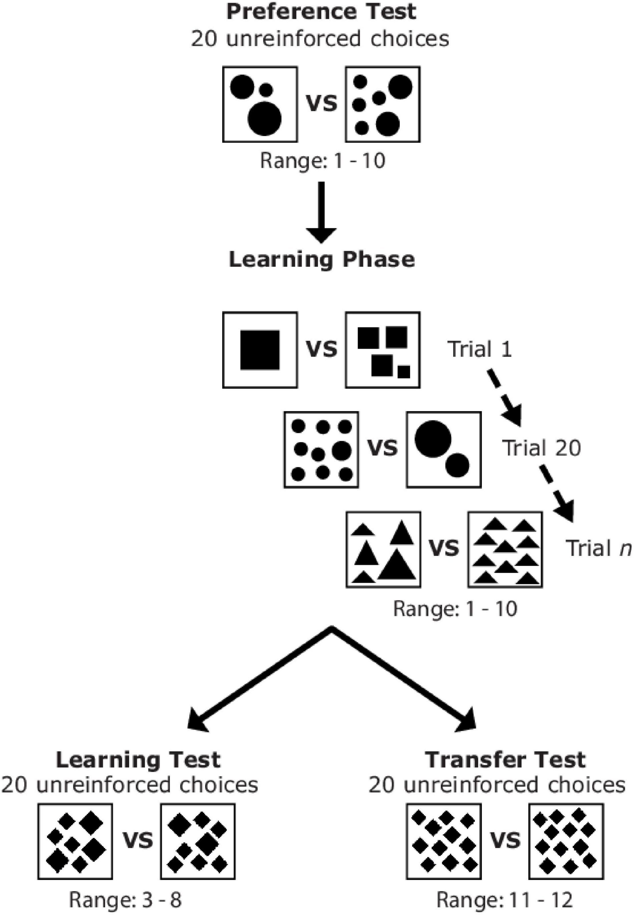
Figure 1 from Howard et al. (2022). Sequence of the different experimental phases and examples of stimuli which could be presented to a bee during the preference test, learning phase, learning test, and transfer test.

Figure 15.1: Figure 1 from Howard et al. (2022). Sequence of the different experimental phases and examples of stimuli which could be presented to a bee during the preference test, learning phase, learning test, and transfer test.

Data from the experiments can be accessed using:

library(Data4Ecologists)
data(beedat)

Key variables in the data set include:

Bee: a unique identifier for each bee
Choice: equal to 1 if the bee made a correct choice and 0 otherwise. For example, a bee trained to prefer even numbers of shapes would have a correct choice if it choose a stimuli with 2, 4, …, 12 shapes.
Test: identifies the type of trial based on whether bees were trained to select even or odd numbers and whether the trial was a learning or transfer test. Test = 1 for learning tests involving even trained bees. Test = 2 for learning tests involving odd trained bees. Test = 3 for transfer tests involving even trained bees. Latly Test = 4 for transfer tests involving odd trained bees.
Ieven: an indicator variable equal to 1 for even trained bees and 0 for odd trained bees
Itransfer: an indicator variable equal to 1 if the observation was from a transfer test and 0 for a learning test

Note: the Test variable should be treated as a factor using:

beedat$Test <- as.factor(beedat$Test)

Use a generalized linear mixed effects model to evaluate: a) if it is easier for bees to learn to find even patterns relative to their ability to discern odd patterns; b) if bees performed better during the learning phase relative to the transfer phase; and c) if bees do better than random at picking the right stimuli. Provide statistical evidence to support your conclusions (e.g., confidence intervals or p-values for appropriate hypothesis tests or comparison of models using AIC). (11 pts)
Using a set of equations, describe the model(s) you fit in part 1. Identify the estimated parameters in R output when using the summary function. (4 pts)
Use your fitted model from 4 to estimate the probability that a “typical bee” trained to select stimuli with an even number of shapes chooses correctly on a transfer test. (3 pts)
Explain why the question in 5 refers to a “typical bee”. (2 pts)

If you are curious, I’ve included a video, below, showing an example transfer trial!

Harder, L. D., & Thomson, J. D. (1989). Evolutionary options for maximizing pollen dispersal of animal-pollinated plants. The American Naturalist, 133(3), 323-344.↩︎