Chapter 15 Generalized Linear Mixed Effects Models

15.1 Exercise 1

Consider the RIKZdat data set from Chapter 2 of the book, which can be accessed using:

library(Data4Ecologists)
data(RIKZdat)

To help with model convergence, we will use a scaled and centered version of NAP. We will also create a new variable exposure.low that combines the lowest two exposure categories using:

library(dplyr)
RIKZdat <- RIKZdat %>% mutate(NAPc = as.numeric(scale(NAP)),
                              exposure.low = case_when(exposure ==  11 ~ 1, exposure < 11 ~ 0))

Alter the code, below, used to fit a linear mixed effects model to the RIKZdat data set from Chapter 2 of the book so that it fits a model where, conditional on the random intercepts (and fixed effect covariates), the data are assumed to be Poisson distributed.

jags.lme.rc<-function(){
  
# Priors for the intercepts
 for (i in 1:n.groups){    
  # To allow for correlation between alpha[i] and beta[i], we need to model their joint (multivariate) distribution 
    alpha[i] <- B[i,1]  # Random intercepts
    beta1[i] <-B[i,2] # Rancom slopes for NAP
    B[i,1:2]~ dmnorm(B.hat[i,], Tau.B[,]) # distribution of the vector (alpha[i], beta[i])
    B.hat[i,1]<-mu.int # mean for intercepts
    B.hat[i,2]<-mu.slope # mean for slopes
 }

 # Hyperpriors for intercepts and slopes
  mu.int ~ dnorm(0, 0.001)       
  mu.slope ~dnorm(0,0.001)
 
 # Hyperpriors for Sigma =  var/cov matrix of the slope/intercept parameters
  sigma.int ~ dunif(0,100) #sd intercepts
  sigma.slope~dunif(0,100) # sd of slopes
  rho~dunif(-1,1) # correlation among intercepts and slopes
  Sigma.B[1,1]<-pow(sigma.int,2)
  Sigma.B[2,2]<-pow(sigma.slope,2)
  Sigma.B[1,2]<-rho*sigma.int*sigma.slope
  Sigma.B[2,1]<-Sigma.B[1,2]
 
 # Tau = inverse of Sigma (analogous to precision for univariate normal distribution)
  Tau.B[1:2,1:2]<-inverse(Sigma.B[,])
 
 # Priors for exposure regression parameter and within individual variance
  beta2 ~ dnorm(0, 0.001)       # Common slope exposure
  tau <- 1 / ( sigma * sigma)       # Residual precision
  sigma ~ dunif(0, 100)         # Residual standard deviation

# Likelihood
 for (i in 1:nobs) {
    mu[i] <- alpha[Beach[i]] + beta1[Beach[i]]*NAPc[i]+beta2*exposure.low[i] # Expectation
    Richness[i] ~ dnorm(mu[i], tau)     # The random variable
 }
}

Describe the model using a set of equations.
Fit the same model using the lmer function in the lme4 package and compare the estimates of the fixed effect and variance parameters.

15.2 Exercise 2

Consider the RIKZdat data set from Chapter 2 of the book, which can be accessed using:

library(Data4Ecologists)
data(RIKZdat)

To help with model convergence, we will use a scaled and centered version of NAP. We will also create a new variable exposure.low that combines the lowest two exposure categories using:

library(dplyr)
RIKZdat <- RIKZdat %>% mutate(NAPc = as.numeric(scale(NAP)),
                              exposure.low = case_when(exposure ==  11 ~ 1, exposure < 11 ~ 0))

Fit a model relating species richness (Richness) to NAP to exposure.low. Include a random intercept for each beach. Assume, conditional on the random intercepts (and fixed effect covariates), that the data are Poisson distributed.
Update the model from step 1 so that it also allows the effect of NAP to vary by beach using a random coefficient model. Why can we not allow the effect of exposure.low to also vary by beach?
Use glmmTMB function in the glmmTMB package with family = nbinom2 to fit the model in step 2 but assuming that the distribution of species richness, conditional on the random effects (and fixed effect covariates) follows a negative binomial distribution.
Compare the 3 models in steps 1-3 using AIC. Evaluate the reliability of the assumptions for the model with the lowest AIC using the check_model function in the performance package. Make sure to comment on the plots - particularly if you see potential assumption violations.
Write down a set of equations to describe the chosen model in step 4.

15.3 Exercise 3

Consider again the data set from exercise 12.4 containing observations of bird species richness in habitat patches classified according to different landscape types (landscape = Agriculture, Bauxite, Forest, or Urban). The data can be accessed using:

library(Data4Ecologists)
data(birds, package = "Data4Ecologists")

It may also help to drop observations with missing species richness data (e.g., when specifying the model using JAGS):

library(dplyr)
birds <- birds %>% filter(is.na(S)!=TRUE)

In Exercise 12.4, we considered the following model:

$\begin{matrix} S_{i} \sim P o i s s o n (λ_{i}) \\ \log (λ_{i}) = β_{0} + β_{1} I (l a n d s c a p e = B a u x i t e)_{i} + β_{2} I (l a n d s c a p e = F o r e s t)_{i} + \\ β_{3} I (l a n d s c a p e = U r b a n)_{i} + β_{4} \log (A r e a)_{i} + β_{5} \log (A r e a)_{i}^{2} \end{matrix}$

However, we noted that each habitat patch was monitored in 3 separate years. In this exercise, we will attempt to address the fact that each patch was observed repeatedly.

Modify the model to include a random intercept for each habitat patch and fit the model using the glmer function in the lme4 package. Compare this model to the Poisson model without a random intercept. Comment on your findings.
Fit the model using JAGS. Note, if you want to compare coefficients in the two models, make sure to use the same parameterization (i.e., either effects or means coding). Also, you will want to make sure to use raw (or orthogonal) polynomials in both models!
Describe the model in step 2 using a set of equations. Make sure to also describe the assumed prior distributions.

15.4 Exercise 4

For this exercise, you will explore differences between subject-specific (conditional) and population-averaged (marginal) means estimated using generalized linear mixed effects models and generalized estimating equations.

Thompson et al. (2016)⁹ counted birds in a set of waterfowl production areas in Minnesota to evaluate the effects of tree removal treatments. For this exercise, we will ignore the treatments and just explore how total counts of woodland birds changed over the course of the study.

The data for this exercise can be accessed using:

library(Data4Ecologists)
data(d.woodall)

Determine the mean number of birds counted in each year across the different waterfowl production areas. This can be accomplished using the code below (you will want to save this output to an R object so you can plot the counts over time in step 6):

d.woodall %>% group_by(year) %>%
  summarize(meancount = mean(total))

## # A tibble: 7 × 2
##    year meancount
##   <dbl>     <dbl>
## 1     0     1.26 
## 2     1     0.896
## 3     2     0.818
## 4     3     0.775
## 5     4     0.686
## 6     5     0.794
## 7     6     0.761

Fit the following generalized linear mixed effect model to the counts of woodland birds:

glmer(total ~ as.factor(year) + (1 | wpa), family = poisson(), data = d.woodall)

Estimate the mean count for a “typical waterfowl production area” in each year (e.g., using the predict function).

Describe the model from step 2 using a set of equations.
Fit two generalized estimating equation models to these same data, first using an independence working correlation structure and then an exchangeable working correlation structure.

You can use the geeglm function in the geepack package:

geeglm(total ~ as.factor(year), id = wpa, data = d.woodall, family = poisson(), corstr = "independence") geeglm(total ~ as.factor(year), id = wpa, data = d.woodall, family = poisson(), corstr = "exchangeable")

Estimate the population mean count (i.e., across the population of waterfowl production areas) in each year (e.g., using the predict function) for both of these models.

Use the model from step 2 and the results from Section 19.7.2 of the book to estimate the (marginal) population mean count in each year.
Compare the observed means from step 1 to the estimated means in steps 2, 4 and 5. Provide an explanation for any observed differences.

15.5 Exercise 5

For this exercise, we will consider data from the following paper (see abstract below):

Dakin and Montgomeric (2014). Deceptive copulation calls attract female visitors to Peacock leks. The American Naturalist 558-564.

Abstract: Theory holds that dishonest signaling can be stable if it is rare. We report here that some peacocks perform specialized copulation calls (hoots) when females are not present and the peacocks are clearly not attempting to copulate. Because these solo hoots are almost always given out of view of females, they may be dishonest signals of male mating attempts. These dishonest calls are surprisingly common, making up about a third of all hoot calls in our study populations. Females are more likely to visit males after they give a solo hoot call, and we confirm using a playback experiment that females are attracted to the sound of the hoot. Our findings suggest that both sexes use the hoot call tactically: females to locate potential mates and males to attract female visitors. We suggest that the solo hoot may be a deceptive signal that is acquired and maintained through reward-based learning.

The data can be accessed using:

library(Data4Ecologists)
data(peacock)

We will use a centered and scaled version of Julian date to make it easier to fit the model and also change some of the character variables to factors. It will also help with interpretation if we change the reference level for the PrePost variable to be Pre using the following code:

# Character to factor variables
peacock$Place <- as.factor(peacock$Place) 
peacock$PrePost <- as.factor(peacock$PrePost )
peacock$DofY <- scale(peacock$DayofYear) # centers and scales this variable
peacock$PrePost <- relevel(peacock$PrePost, ref = "Pre") # ensures the reference level is "pre hoot"

Use ggplot to explore how the probability of a female being located within 5m of a focal male depends on Julian date, site (i.e., place), and if the observation took place before or after the male produced a hoot call.

library(ggplot2)
library(ggthemes) #colorblind pallete
ggplot(peacock, aes(x = DayofYear, y = FemaleVisit.5m, colour = PrePost)) +
     geom_point(position = position_jitter(w = 2, h = 0.05), size=3) +
     geom_smooth(method="glm",  method.args = list(family = "binomial"))  + 
     facet_wrap(~Place, scales="free") +  scale_colour_colorblind()

## `geom_smooth()` using formula = 'y ~ x'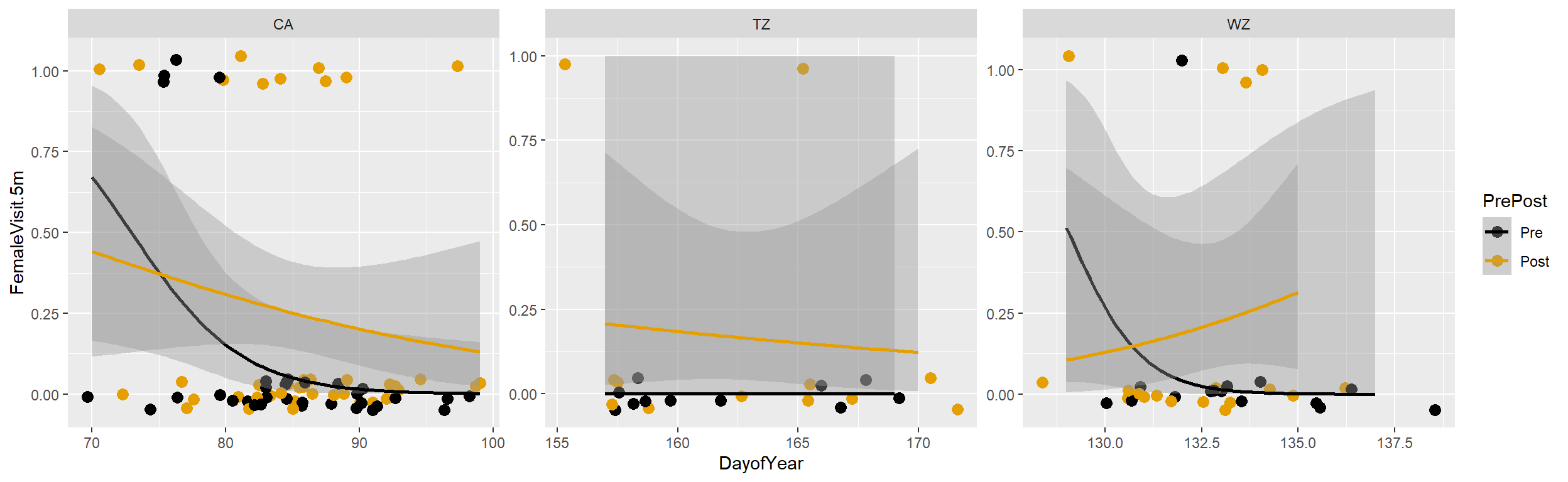

Use the glmer function in the lme4 library to fit a generalized linear mixed effects model in which the log odds of a male attracting a female is modeled as a linear function of Julian date (DofY), site (i.e., Place), and whether the observation period occurred before or after a hoot call (PrePost). Include a random intercept for each male (MaleID).
Interpret the fixed effects parameters and the variance parameter reported by the summary function.
Use the confint function to get profile-likelhood based and Wald-based (i.e., $\pm 1.96 S E$ ) confidence intervals. See ?confint.merMod for the correct syntax. (Note: bootstrap and profile-likelihood based intervals should be “better” than Wald intervals, but there are tradeoffs in terms of time required to get an answer. I tried to include bootstrap confidence intervals when producing the answer key, but it took so long I eventually stopped the computation!).
Fit the same model using JAGS.[Optional: assess goodness-of-fit using Pearson residuals.]. The MCMC samples will be highly autocorrelated so it is important to run the model for longer than most of the examples we have looked at to date. Run the sampler for 80,000 iterations, with a burn-in of 10,000 iterations. Again, use 3 chains but this time with thin = 3 (keep every 3rd observation). Assess convergence using traceplots, density plots, and Gelman-Rubin statistic (R).
Use the geeglm function in the geepack library to fit a generalized estimating equations model in which logit(p) is modeled as a linear function of date, site, and pre- versus post-hoot. Try both independence and exchangeable working correlation structures. In both cases, add an argument scale.fix = TRUE so that R does not estimate an overdispersion parameter.
Describe/interpret the parameters in the GEE model (fit with geepack). Note: interpretation is the same for both working correlation structures, so you only need to do this once!
Compare 95% confidence intervals from both GEE models (with working independence and ex- changeable correlation structures) to 95% credible intervals for the glmm (fit using JAGS) and 95% confidence intervals (profile-likelhood and Wald-based) you calculated using confint and glmer. Comment on your findings. HINT: you can access the standard errors for the coefficients in the gee model using coef(summary([name of gee model]))$Std.err. You can then get Wald-based intervals by taking $\pm 1.96 S E$ .

15.6 Exercise 6

For this exercise, you will consider a data set from Howard et al. (2022).

Howard, S. R., Greentree, J., Avarguès-Weber, A., Garcia, J. E., Greentree, A. D., & Dyer, A. G. (2022). Numerosity Categorization by Parity in an Insect and Simple Neural Network. Frontiers in Ecology and Evolution, 252.

The authors of this study evaluated whether: 1) free-flying honeybees could be trained to differentiate between odd and even numbers of geometric shapes, and 2) whether they could transfer this learning to new situations. Bees were initially trained to prefer odd or even numbers of shapes by associating stimuli (cards with 1-10 shapes) with either sugar or quinine. After training, each bee participated in 20 learning-test trials in which they made a choice between stimuli with an even or odd number of shapes. These trials again used stimuli with between 1 and 10 shapes. Lastly, each bee also participated in 20 transfer-test trials where they chose between stimuli consisting of either 11 or 12 shapes. The full experimental design is illustrated in the figure below and more details can be found in the paper if you are interested.

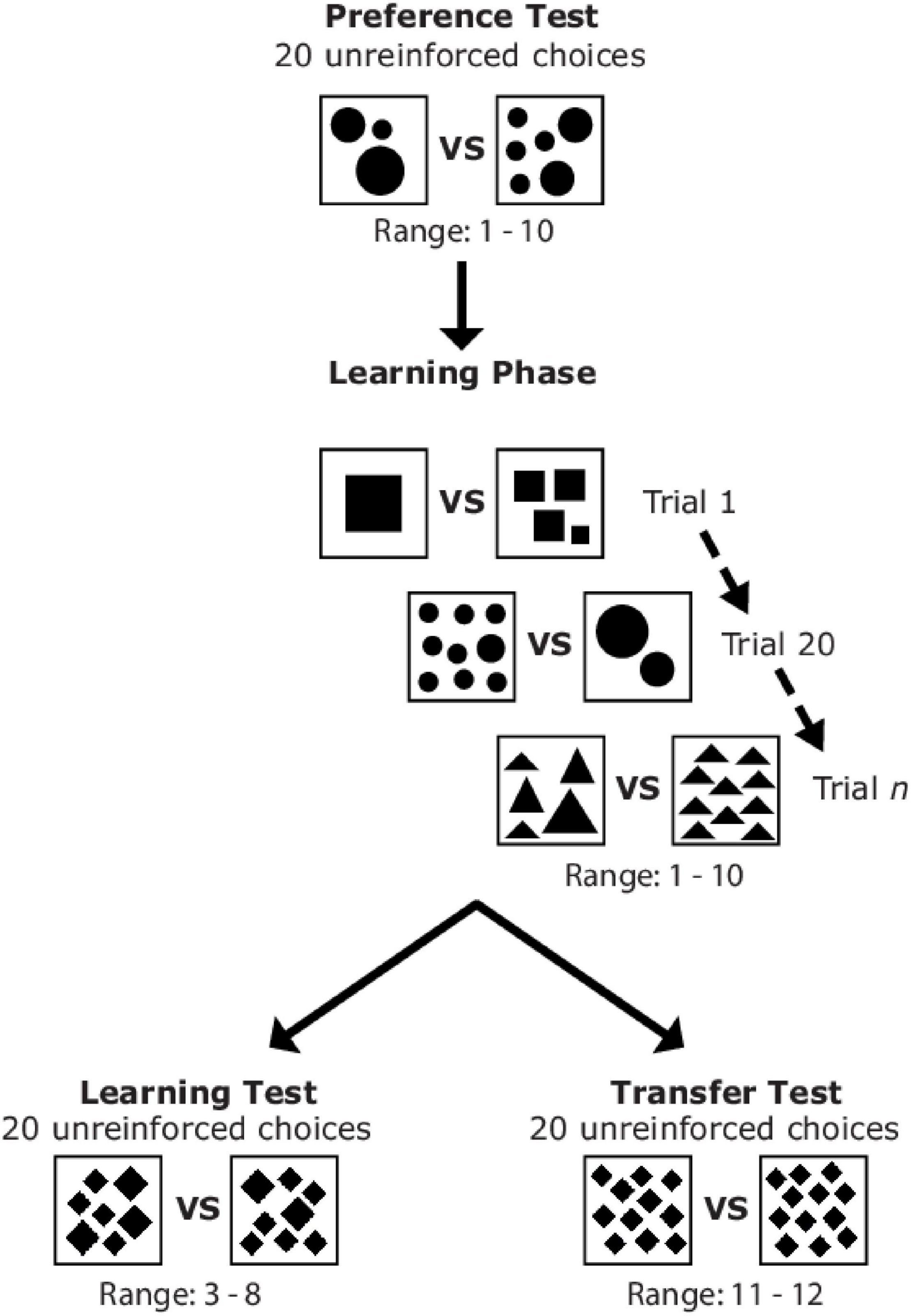
Figure 1 from Howard et al. (2022). Sequence of the different experimental phases and examples of stimuli which could be presented to a bee during the preference test, learning phase, learning test, and transfer test.

Figure 15.1: Figure 1 from Howard et al. (2022). Sequence of the different experimental phases and examples of stimuli which could be presented to a bee during the preference test, learning phase, learning test, and transfer test.

Data from the experiments can be accessed using:

library(Data4Ecologists)
data(beedat)

Key variables in the data set include:

Bee: a unique identifier for each bee
Choice: equal to 1 if the bee made a correct choice and 0 otherwise. For example, a bee trained to prefer even numbers of shapes would have a correct choice if it choose a stimuli with 2, 4, …, 12 shapes.
Test: identifies the type of trial based on whether bees were trained to select even or odd numbers and whether the trial was a learning or transfer test. Test = 1 for learning tests involving even trained bees. Test = 2 for learning tests involving odd trained bees. Test = 3 for transfer tests involving even trained bees. Latly Test = 4 for transfer tests involving odd trained bees.
Ieven: an indicator variable equal to 1 for even trained bees and 0 for odd trained bees
Itransfer: an indicator variable equal to 1 if the observation was from a transfer test and 0 for a learning test

Note: the Test variable should be treated as a factor using:

beedat$Test <- as.factor(beedat$Test)

Use a generalized linear mixed effects model to evaluate: a) if it is easier for bees to learn to find even patterns relative to their ability to discern odd patterns; b) if bees performed better during the learning phase relative to the transfer phase; and c) if bees do better than random at picking the right stimuli. Provide statistical evidence to support your conclusions (e.g., confidence intervals or p-values for appropriate hypothesis tests or comparison of models using AIC). (11 pts)
Using a set of equations, describe the model(s) you fit in part 1. Identify the estimated parameters in R output when using the summary function. (4 pts)
Use your fitted model from 4 to estimate the probability that a “typical bee” trained to select stimuli with an even number of shapes chooses correctly on a transfer test. (3 pts)
Explain why the question in 5 refers to a “typical bee”. (2 pts)

If you are curious, I’ve included a video, below, showing an example transfer trial!

15.7 Excersise 7

For this exercise, you will consider a data set from Brandell et al. (2021ab):

Brandell, Ellen E (2021a). Serological dataset and R code for: Patterns and processes of pathogen exposure in gray wolves across North America Dataset. Dryad. https://doi.org/10.5061/dryad.5hqbzkh51.

Brandell, Ellen E. et al. (2021b), Patterns and processes of pathogen exposure in gray wolves across North America, Scientific Reports, Journal-article, https://doi.org/10.1038/s41598-021-81192-w.

The data can be accessed using:

library(Data4Ecologists)
library(lme4)
data("WolfPathogen")

For this exercise, we will explore generalized linear mixed effects models for predicting the infection status of wolves with respect to canine parvovirus-2, captured in the cpv.binary variable (coded as a 1 if the wolf tested positive for the disease and 0 otherwise). We will consider the following predictor variables:

age.cat = wolf age class; P = Pup (<1 year old), S = subadult (1-2 years old), and A = adult (great than or equal to 3 years old).
sex = sex of the wolf; F = Female, M = Male
year = year of the observation
pop = ID representing the study population for each wolf

Note, the wolves included in this study come from 17 different study populations (represented in the popvariable), and thus, the observations may not be independent unless our predictor variables fully account for the differences in prevalence among the populations.

table(WolfPathogen$pop)

## 
##  AK.PEN BAN.JAS      BC  DENALI   ELLES    GTNP  INT.AK MEXICAN      MI      MT 
##     100      96     145     154      11      60      35     181     102     351 
##   N.NWT     ONT   SE.AK     SNF  SS.NWT     YNP    YUCH 
##      67      60      10      92      34     383     105

Before beginning the exercise, create a new variable, yearc, that ranges from 0 to 27 (rather than 1992 to 2019).

WolfPathogen$yearc <- WolfPathogen$year - min(WolfPathogen$year)

Begin by fitting a model that includes a random intercept for pop and that includes the variables age.cat, sex, and yearc. Here, yearc will account for an overall downward trend in infection rates over time.
Describe the model using a set of equations. Match all parameters in the equations to estimates of the parameters in the above output.
Interpret plogis( $β_{0}$ ), where $β_{0}$ is the intercept in the model if you use reference coding for the categorical variables.
Interpret the coefficients for sexM and yearc in terms of their effects on the odds of infection.
Predict the probability of infection for a male, subadult wolf from a “typical population” when yearc = 0.
Perhaps a yearly trend (on the logit scale) is not sufficient for capturing changes in infection status over time. Fit a model with a quadratic polynomial for yearc (using orthogonal polynomials, the default when using poly). Compare this model to the original model using a likelihood ratio test (e.g., using anova(mod1, mod2)). What do you conclude?
Instead of modeling yearc as a continuous variable (with linear or quadratic effect), we could treat yearc as a categorical variable.

table(WolfPathogen$year)

## 
## 1992 1993 1994 1995 1996 1997 1998 1999 2000 2001 2002 2003 2004 2005 2006 2007 
##    5    3    5    6    6   25   22   33   46   31   31   55   50   64  120  128 
## 2008 2009 2010 2011 2012 2013 2014 2015 2016 2017 2018 2019 
##  129  106  122  123   95  105   89   80  114  126  226   41

Given the large number of categories, it probably makes most sense to include year as a random effect. Consider the model below and describe how it treats the statistical dependencies for different observations (from the same population, same year, same population and same year).

mod3 <- glmer(cpv.binary ~ age.cat + color + sex + (1|pop)+ (1|year), 
        data=WolfPathogen, 
        family=binomial())
summary(mod3)

## Generalized linear mixed model fit by maximum likelihood (Laplace
##   Approximation) [glmerMod]
##  Family: binomial  ( logit )
## Formula: cpv.binary ~ age.cat + color + sex + (1 | pop) + (1 | year)
##    Data: WolfPathogen
## 
##      AIC      BIC   logLik deviance df.resid 
##   1079.9   1116.3   -532.9   1065.9     1326 
## 
## Scaled residuals: 
##     Min      1Q  Median      3Q     Max 
## -7.4454  0.0671  0.2348  0.4772  3.8603 
## 
## Random effects:
##  Groups Name        Variance Std.Dev.
##  year   (Intercept) 0.5795   0.7612  
##  pop    (Intercept) 2.8775   1.6963  
## Number of obs: 1333, groups:  year, 28; pop, 16
## 
## Fixed effects:
##             Estimate Std. Error z value Pr(>|z|)    
## (Intercept)  2.30649    0.53798   4.287 1.81e-05 ***
## age.catP    -2.46855    0.29150  -8.468  < 2e-16 ***
## age.catS    -0.86413    0.20674  -4.180 2.92e-05 ***
## colorG      -0.03978    0.20204  -0.197    0.844    
## sexM         0.10648    0.16058   0.663    0.507    
## ---
## Signif. codes:  0 '***' 0.001 '**' 0.01 '*' 0.05 '.' 0.1 ' ' 1
## 
## Correlation of Fixed Effects:
##          (Intr) ag.ctP ag.ctS colorG
## age.catP -0.231                     
## age.catS -0.192  0.420              
## colorG   -0.267 -0.003 -0.022       
## sexM     -0.162 -0.027  0.055  0.014

Thompson, S. J., Arnold, T. W., Fieberg, J., Granfors, D. A., Vacek, S., and Palaia, N. (2016). Grassland birds demonstrate delayed response to large‐scale tree removal in central North America. Journal of Applied Ecology, 53(1), 284-294.↩︎