Chapter 17 Final Exam 2024
17.1 Exercise 1
The Environmental Protection Agency (EPA) provides publicly available data sets online through their National Aquatic Resource Surveys (NARS) Data Download Tool (https://owshiny.epa.gov/nars-data-download/). In this exercise, we will use a subset of data from the NARS Data Download Tool that reports mercury concentrations in various fish species collected across a number of states from 2018 to 2019.
We will focus on six fish species that are well represented in this data set and have varying diets; brown trout and brook trout (Salmonidae family), largemouth bass and smallmouth bass (Centrarchidae family), channel catfish (Ictaluridae family), and white sucker (Catostomidae family).
Data citation:
U.S. Environmental Protection Agency. (2021). National Aquatic Resource Surveys. Rivers and Streams, Fish Tissue (Plugs) - Mercury 2018/2019 (data and metadata files). Available from U.S. EPA website: http://www.epa.gov/national-aquatic-resource-surveys/data-national-aquatic-resource-surveys. Date accessed: 2024-02-24.
The data can be accessed using the Data4Ecologists package. You may need to update the package before you can access the data. To update the package, type: devtools::install_github("jfieberg/Data4Ecologists")
Then, we can access the data using:
The dataset contains the following variables:
species= specieslength= length of fishHg= mercury concentrationstate= State where the sample was taken
Fit a linear model relating mercury concentration to
lengthandspecies. Use effects/reference coding forspecies. Describe the model using a set of equations and interpret the model parameters in the context of the problem. Do not forget about . (6 pts)Write down the design matrix for the first 3 observations shown below (3 pts):
##           species length     Hg state
## 1 largemouth bass    390 0.2730    OK
## 2 channel catfish    350 0.0889    OK
## 3     brook trout    177 0.1200    WI
Fit the same model but using means coding. Again, write down the design matrix for the first 3 observations (3 pts).
Evaluate whether or not you think the assumptions of linear regression are met. Justify your answers by referring to characteristics in appropriate diagnostic plots. (4 pts)
Modify the model from part 1 to allow the variance to depend on the species of fish. Keep the model for the mean the same (i.e., assume that the mean mercury level depends on the species and length of the fish). Save the model to an object named
mod3. (3 pts)Write down a set of equations that describes the distribution of mercury observations for channel catfish as a function of their
lengthbased on your assumed/fitted model. I.e., I would like to see: 1) the assumed statistical distribution; 2) the parameters of that statistical distribution written as a function of predictor variables, but where these expressions are simplified by defining the model just for channel catfish. Lastly, I want you to plug in estimates of any statistical parameters (e.g., from the output created from thesummaryfunction applied to your fitted model). (4 pts)Add the Pearson residuals and the fitted values () from the gls model in step 6 to the original data set using the following code:
library(dplyr)
Fish_Mercury2 <- Fish_Mercury %>% mutate(fitted = mod3$fitted, pearsonr = residuals(mod3, type = "pearson"))
Consider the residual plots constructed using the code below. What do they tell us about the linearity assumption and the assumed variance model? What would we hope to see if the assumptions were met? (4 pts):
17.2 Exercise 2
For this problem, we will again consider the Fish_Mercury data set, which we can access using:
We will also use the following packages:
In the first problem set, we used Generalized Least Squares to try to meet the model assumptions. Here, we will instead consider a model for log-transformed mercury concentrations. Use the code below to add logHg to the data set:
Fit a linear model, using reference / effects coding, to predict log mercury concentration from
lengthandspecies. Evaluate whether or not you think the assumptions of linear regression are met for the model in step 1. (4 pts)Show how we can estimate the logHg concentration of a white sucker that is 285 mm long using the coefficients from the fitted model. (3 pts)
What if we want to estimate the mean Hg of white suckers that are 285mm in length (rather than the mean of log(Hg))? It turns out that back-transforming the prediction for the log(Hg) concentration will estimate the median Hg concentration rather than the mean concentration. To estimate the mean, we have to use:
- is the estimated mean on the log scale.
- describes the estimated variability of the observations/errors (recall, the summary function applied to our fitted model will return an estimate of ; we just need to square it to get ).
For this part of the problem, I want you to use simulations to demonstrate these results. (4 pts)
Specifically:
A. Use rnorm to simulate 500,000 observations of log(Hg) from the fitted model with length = 285 and species = white sucker. I.e., generate new responses using: where the are generated using the rnorm function with from the fitted model. Store these results for use in step B and C, below.
B. Transform the observations from step (A) back to the original scale to provide simulated observations of Hg. I.e., take the stored values from step a and exponentiate them using the exp() function in R.
C. Calculate the mean and median of the simulated Hg values from step B. Compare these values to what you get when you back-transform your answer from part 3 of this problem using exp().
Switching gears, what if we also wanted to account for variation in mercury level that may be attributable to geographical differences captured by
state? We could fit a linear model withstateincluded (similar to how we modeled differences amongspecies). Alternatively, we could fit a mixed-effects model with random intercepts for each state. Supply the necessary R code to fit both models. (3 pts)Reflect on the advantages and disadvantages of the two modeling approaches (i.e., the mixed-effects model fit using
lmerand the fixed-effects model usinglm). How do they differ? Which approach do you generally favor and why? Does your answer depend on your modeling objective? Note, there is not necessarily a right answer here. (4 pts)
17.3 Exercise 3
For this exercise, we will explore data from:
Chenoweth, E. M., Straley, J. M., McPhee, M. V., Atkinson, S., & Reifenstuhl, S. (2017). Humpback whales feed on hatchery-released juvenile salmon. Royal Society Open Science, 4(7), 170180.
They collected data on the presence/absence of humpback whales near hatchery sites where juvenile salmon were periodically released. The data set can be loaded using (again, you may need to update the Data4Ecologists package):
The data set contains the following variables:
Date= Date of observationYear= Year of observationHatchery= Hatchery where observation was made (there were five release sites: HiddenFalls, Takatz, Mist Cove, Little Port Walter and Port Armstrong)DOY= Day of yearTiming= categorical variable indicating whether the observation was during a period before, during, or after salmon were released from the hatchery.Observed= 1 if humpback whales were observed and 0 otherwiseduration= the total duration of sampling effort associated with each observation period
We will also make use of the following packages:
library(lme4) # for glmms
library(MASS) # for mvrnorm function
library(dplyr) # for data wrangling
library(ggeffects) # for effect estimation/plotting
The authors describe one of the models they fit, below (note that site is equivalent to Hatchery in the data set):
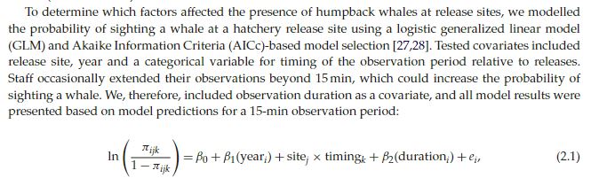
Suggest 2 improvements to their model equation that are NOT related to how the effects of
year,Hatchery,Timing, anddurationare described. Hint 1: Distribution? Hint 2: ? (4 pts)Fit the above logistic regression model as well as a reduced model without the interaction between
HatcheryandTiming. Use tools (e.g., Likelihood Ratio Tests, AIC) we have discussed in class to compare the two models. Which model do you prefer? Justify your answer (4 pts)
- Consider a GLMM where the probability of observing humpback whales is modeled as a function of
Timinganddurationbut whereHatcheryandYearare both modeled using random effects (i.e., eachHatcheryand eachYearare given their own random intercepts). Describe the model using a set of equations, and match the parameters in your equations to those in the output generated by thesummaryfunction. (4 pts)
To make it easier to fit the model, we will want to replace duration with a scaled and centered version created using the code below (i.e., use duration.sc in your GLMM):
We can then fit the model using:
mod3 <- glmer(Observed ~ Timing + duration.sc +(1|Hatchery) + (1|Year),
              data=HatcheryObs, family = binomial())
summary(mod3)
## Generalized linear mixed model fit by maximum likelihood (Laplace Approximation) ['glmerMod']
## Family: binomial ( logit )
## Formula: Observed ~ Timing + duration.sc + (1 | Hatchery) + (1 | Year)
## Data: HatcheryObs
##
## AIC BIC logLik deviance df.resid
## 883.9 918.2 -436.0 871.9 2246
##
## Scaled residuals:
## Min 1Q Median 3Q Max
## -0.9457 -0.2846 -0.1738 -0.1209 10.5523
##
## Random effects:
## Groups Name Variance Std.Dev.
## Year (Intercept) 0.09235 0.3039
## Hatchery (Intercept) 0.60444 0.7775
## Number of obs: 2252, groups: Year, 6; Hatchery, 5
##
## Fixed effects:
## Estimate Std. Error z value Pr(>|z|)
## (Intercept) -2.95858 0.44915 -6.587 4.49e-11 ***
## TimingBeforeRelease -1.62108 0.43554 -3.722 0.000198 ***
## TimingDuringRelease 0.41707 0.31139 1.339 0.180453
## duration.sc 0.22975 0.05476 4.195 2.72e-05 ***
## ---
## Signif. codes: 0 '***' 0.001 '**' 0.01 '*' 0.05 '.' 0.1 ' ' 1
##
## Correlation of Fixed Effects:
## (Intr) TmngBR TmngDR
## TimngBfrRls -0.370
## TmngDrngRls -0.506 0.626
## duration.sc -0.005 -0.118 -0.075Interpret the fixed effects parameters in the model (4 pts). Correct interpretation on the log-odds scale will earn 3 of the 4 points. For full credit, interpret one or more of the parameters in terms of effects on the odds of presence.
Use the coefficients from the model and
plogisto predict the probability of seeing a whale at a “typical” hatchery, during a “typical” year, whenduration.sc= 0, before, during, and after a release of juvenile salmon (i.e., I would like to see 3 predictions). (4 pts)
Note, one way to check your answer would be to use the ggeffect function in the ggeffects package. This will also provide confidence intervals to go with these estimated probabilities.
17.4 Exercise 4
In this exercise, we will explore data from:
Chakrabarti, S., Jhala, Y. V., Dutta, S., Qureshi, Q., Kadivar, R. F., & Rana, V. J. (2016). Adding constraints to predation through allometric relation of scats to consumption. Journal of Animal Ecology, 85(3), 660-670.
The lead author, Dr. Stotra Chakrabarti is currently a professor at Macalester College and did a postdoc with Dr. Joseph Bump in the Department of Fisheries, Wildlife, and Conservation Biology here at the University of Minnesota.
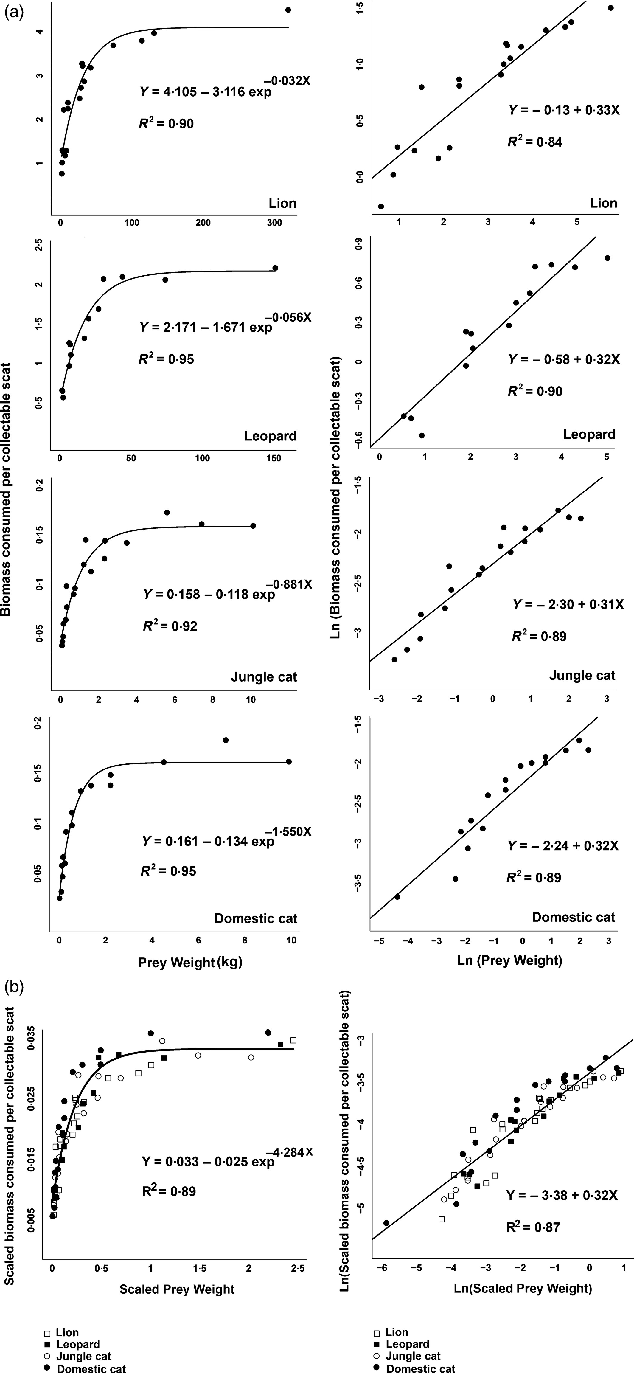
In the paper, Chakrabarti et al. parameterized biomass models that can be used to estimate the biomass of consumed prey from scat collected in the field. To do so, they used feeding trials where a variety of predators were fed prey of different sizes. They then measured how much biomass was consumed per collectible scat that was recovered after the feeding trial.
The data are again contained in the Data4Ecologists package and can be accessed using:
The data set contains the following variables:
Predator= Predator consuming prey in the feeding experimentPrey.number= Type of prey and number of prey consumed in feeding trialMean_prey_wt= Mean weight (kg) of the prey species being offered during feeding trialBiomass.per.scat= Biomass (kg) consumed per collectable scat
Will will make use of the following packages:
library(dplyr) # for data wrangling
library(ggplot2) # for plotting
library(R2jags) # for fitting models using JAGS
library(MCMCvis) # for visualizing MCMC output
library(mcmcplots) # for denplot and traplot for inspecting MCMC output
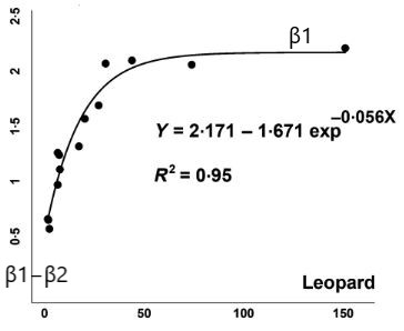
library(ggthemes) # for colorblind palleteFor this exercise, we will build a biomass model for predicting prey biomass consumed (Biomass.per.scat) based on the mean weight of the prey species (Mean_prey_wt). We will only consider the observations from feeding trials involving leopards:
Our goal is to replicate the analysis of the Leopard data shown in Figure 1 from Chakrabarti et al. (shown below), and to add confidence and (ideally) prediction intervals to the plot.
17.4.0.1 Assumed Statistical Model
It is helpful to consider the fitted line as describing the mean Biomass per scat, , as a function of mean prey weight, :
To estimate the parameters and also obtain a confidence interval for , we could use either Maximum Likelihood or Bayesian inference.
To accomplish our goals using Maximum Likelihood, we would need to:
- Specify the likelihood for the data.
- Estimate the parameters that maximize the likelihood using something like
optim. This would also require us to specify starting values for the numerical optimization routine. - We would need to use the delta method to quantify the variance in our function. Alternatively, we could use bootstrapping to get a confidence interval.
As a Bayesian, we would need to:
- Specify the likelihood for the data.
- Specify priors for all of our parameters.
- Use MCMC to obtain posteriors for all of our parameters.
- Use the posterior distributions of our parameters to form posterior distributions of for different values of (i.e.,
Mean_prey_wt).
Either way, we need a likelihood and some understanding of the possible values that the parameters can take on. Let’s assume our biomass measurements are Normally distributed with constant variance. This gives us the following model:
where again, refers to the observations of Biomass.per.scat and to the Mean_prey_wt measurements.
Note that:
- if we set to , .
- if we set to , .
Thus, is the asymptote of the curve and has to be . And, we can estimate as the difference between the y-intercept and (note, also has to be ). Lastly, describes how fast we approach the asympotote, and it must also be .
- I’ve created a skeleton JAGS function, below, where I’ve used this information to specify 3 uniform priors for the model parameters. Fill in any missing information and fit the model. Make sure that you write the likelihood using the same names as supplied in the
jags.dataobject that I created. (5 pts)
biomassmod<-function(){

# Priors for mean
beta1 ~ dunif(0, 10)
beta2 ~ dunif(0, 10)
beta3 ~ dunif(0, .1)
sigma ~ dunif(0, 3)
tau <-

# Likelihood
  for(i in 1:n){

    mu[i]
  }
 }

# Bundle data
jags.data <- list(biomass = leoparddat$Biomass.per.scat, preywt = leoparddat$Mean_prey_wt, n = nrow(leoparddat))

#' Parameters to estimate
params <- c("beta1", "beta2", "beta3", "mu", "sigma")

# MCMC settings
nc = 3
ni = 10000
nb = 3000
nt = 1

# Start Gibbs sampler
jagsscat <- jags(data = jags.data,
                parameters.to.save = params,
                model.file = biomassmod,
                n.thin = nt,
                n.chains = nc,
                n.burnin = nb,
                n.iter = ni,
                progress.bar="none")
Make sure to evaluate whether you MCMC samples have converged in distribution. If you are unable to get JAGS to run, describe how you would accomplish this step. (4 pts)
Plot the data, along with 95% credible intervals for the . (4 pts)
Extra credit: generate and plot 95% prediction intervals. Hint: to accomplish this goal, we could have JAGS generate new data (formally, posterior predictions) similar to the step we have used in our Bayesian goodness-of-fit tests. (3 pts extra)
For extra hints on steps 3 and 4, you might want to revisit Sections 13.5 and 13.6 of the book.