Chapter 5 Generalized Least Squares (GLS)
5.1 Exercise 1
This first exercise will consider data collected by Eric North, an urban forester who took my class the first or second year I taught it. Some of Eric’s masters research was aimed at predicting damage to sidewalks from boulevard trees planted between the curb and sidewalk (North, Johnson, & Burk, 2015). The degree of damage largely depends on how much the trunk of the tree spreads out (measured by “trunk flare” Figure 5.1 right), which can be predicted from measures of the diameter at breast height (Figure 5.1 left).
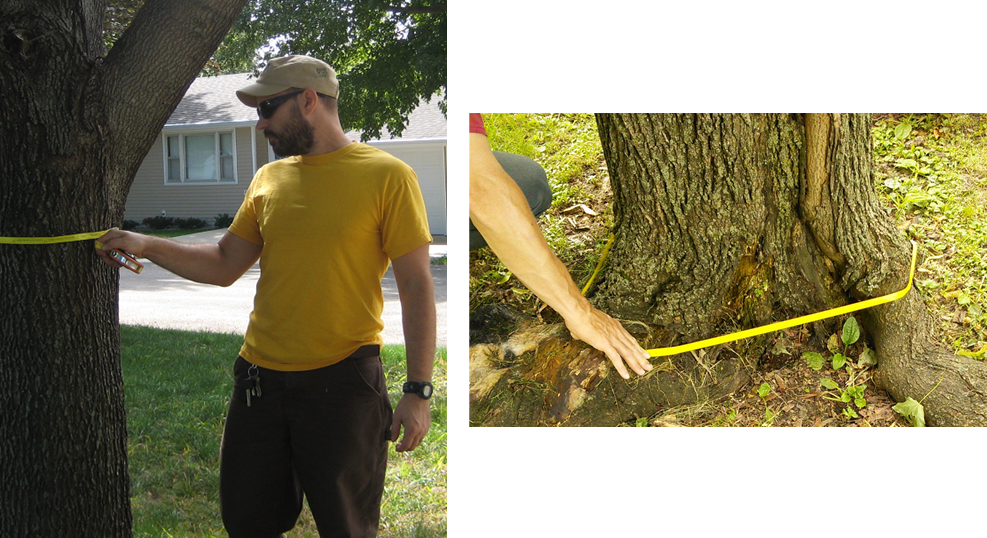
Figure 5.1: Measurements of truck flare diameter (right photo) and diameter at breast height (DBH, left photo).
We will explore linear models relating trunk flare circumference () to diameter at breast height (). As noted by Hilbert et al. (2020) and North et al. (2015), there are several potential uses of this type of model, including:
- determining planting space needed for trees based on their potential size
- identifying areas where there might be current or future damage to infrastructure due to tree roots
- estimating stump size for cost estimates associated with stump removal.
The data for this set of exercises is contained in the Data4Ecologists package and can be accessed using:
- Subset the data to include only Acer saccharinum (Species = 4; sugar maple).
- Fit a linear model relating trunk flare () to diameter at breast height () using
lm. Evaluate the assumptions of the model using residual plots. - Fit a model where the variance is assumed to increase with
dbhusing thevarPowerfunction. - Describe the fitted GLS model using a set of equations. Match the parameters in your equations to the output generated using the
summaryfunction applied to your fitted GLS model.
- Create a plot of Pearson residuals, versus (you can use
plot(modelname)to accomplish this task). Comment on whether you think the GLS model is appropriate. - Use AIC to compare the fit of the standard linear model and the fit of the GLS model (use
AIC(model1, model2), wheremodel1andmodel2are the names you assign to the two fitted models). Before making this comparison, refit the linear model usinggls(this will ensure both models are fit using “REML”, which will be discussed in a later chapter). Which model appears to give the better fit (note: lower AIC is “better”)? - Inspect the estimated regression coefficients and their standard errors. Do they change much when you account for non-constant variance?
5.2 Exercise 2
This exercise was contributed by Anu Li, who took FW8051 in the spring 2024.
The data for this exercise come from a Le Sueur River Basin sediment characterization project carried out by then-graduate student at the University of Minnesota, Anna Baker, Professor Jacques Finlay, and others from 2015-2018. We will consider a subset of the data in this data repository (Baker et al., 2019). Specifically, we will focus on three variables contained in the data set:
Type= Type of sediment/erosional sourceP= Sediment phosphorus concentration, in milligrams per kilogram of sieved fine sedimentSRP= Water extractable soluble reactive phosphorus concentration, in milligrams per kilogram of sieved fine sediment
The latter two variables were renamed (from P (mg/kg) <63 µm and Water Extractable SRP (mg/kg) <63µm, respectively) to make the data easier to read into R. In addition, cases with missing values for either phosphorus measurement have been dropped.
Soluble reactive phosphorus (SRP) is a biologically-available form of phosphorus that causes eutrophication when found in excess in water. Phosphorus can be measured using many different methods, some of which are costly, and none of the methods are perfect. Let’s see if we can predict SRP from phosphorus in the sediment, focusing on the fine particle fraction, defined as having a diameter less than 63 microns.
To complete this exercise, you will want to load the following packages:
You can access the data using:
Fit a linear regression model using
P(x-axis) to predictSRP(y-axes). Plot the data with the regression line overlayed. Also, use thesummaryfunction to inspect the fitted model.Check the linear model assumptions graphically and evaluate whether they appear reasonable.
Fit a model in which the variance is assumed to increase with phosphorus in the sediment,
P, using thevarPowerfunction. Use thesummaryfunction to inspect the model.Write out equations that describe the fitted GLS model. Match parameters to the output from the summary function.
Create a plot of the Pearson residuals versus fitted values using plot(
modelname). Is the variance model appropriate for the data?Sediment and soil samples were collected from different points in the basin, such as bluffs, stream banks, and agricultural sites (captured in the variable,
Type). Fit a power variance model for the same response and predictor variables, except this time allow the variance parameters to depend on each level of the categorical valueType.Write out equations for calculating the variance for
Type=AgandType=SB, replacing the parameters with their estimates from the output of thesummaryfunction.Create a plot of the Pearson residuals versus fitted values for this model. Is the variance model appropriate for the data?
Compare the AIC of all three models (linear, power variance, and power variance with
Type) using AIC(model 1, model 2, model 3). To do this, you must recreate the linear model using gls instead of lm. Given a low AIC indicates a better fit, which model is best for these data?Plot all 3 regression lines on the same plot and also overlay the data. The easiest way to do this is to append predictions from each model on the original data frame and then use ggplot with 3 separate calls to geom_line. How do the models differ? Why do you think they differ in this way? Hint: GLS models will result in larger weights associated with observations that are assumed to be less variable.