Chapter 9 Introduction to Probability Distributions
9.1 Exercise 1
This exercise will consider the 4 basic functions used to work with distributions in the context of the Normal distribution with mean 0 and standard deviation 1. The functions are named dnorm, pnorm, qnorm, rnorm and are depicted in Figure 9.1.
![Figure from (Jack Weiss’s class notes)[https://sakai.unc.edu/access/content/group/3d1eb92e-7848-4f55-90c3-7c72a54e7e43/public/docs/lectures/lecture13.htm] depicting the 4 basic probability functions for working with the Normal distribution in R.](09-ProbabilityDistributions_files/figure-html/distsR-1.png)
Figure 9.1: Figure from (Jack Weiss’s class notes)[https://sakai.unc.edu/access/content/group/3d1eb92e-7848-4f55-90c3-7c72a54e7e43/public/docs/lectures/lecture13.htm] depicting the 4 basic probability functions for working with the Normal distribution in R.
Assume women’s heights follow a normal distribution with mean of 64 inches and standard deviation 3 inches. Assume men’s heights follow the same distribution but with an average of 70 inches. Use R to:
Find the probability that a randomly chosen female is less than 60 inches tall.
Find the probability a randomly chosen male is at least 72 inches tall.
Find the height, x, such that only 2% of females are shorter than x.
Find the proportion of males between 68 and 71 inches tall.
Plot the distributions for both males and females (i.e., both normal distributions) on the same plot. You can do this by:
- Creating an object, x, that spans a range of heights, e.g.,
x <-seq(50,80, length=1000). - Using
plot(x, dnorm(x, mean= , sd = ))for the first density andlines(x, dnorm(x, mean=, sd = ))for the second. Or, using the curve function twice (withadd=TRUE) for the second density (e.g.curve(dnorm(x, mean=, sd=), from=50, to=80).
- Generate 5000 random male heights and 5000 random female heights. Combine the data and create a smooth histogram of the simulated heights using the density function. Does the distribution appear to be Gaussian?
9.2 Exercise 2
The Minnesota DNR decides to monitor various wildlife species using remotely triggered camera traps. Cameras are set up at various locations throughout the state. When an animal passes in front of the camera, the camera is “triggered”, and a picture of the animal is recorded. Assume the number of pictures of white-tailed deer recorded in a week can be described by a negative binomial distribution with and (note, is referred to as size in R’s dnbinom function). Use dnbinom, qnbinom, rnbinom, and pnbinom to answer the following questions:
- What is the probability that a camera trap catches at least 1 deer in a week?
- What is the probability that a camera trap catches between 3 and 5 deer in a week?
- Calculate the number of pictures of deer in a week, , such that 90% of the camera traps record fewer pictures than .
- Simulate a data set with 100 different camera traps (with a negative binomial distribution and parameters and ). Compare the distribution of the simulated data to the negative binomial distribution with = 3 and = 1. You can adapt methods used in class to do this - or consider using the following steps:
Create a histogram using the
histfunction in R, but make sure to include the argumentprobability=TRUE. To make sure everything lines up correctly, I also recommend using the breaks argument to make sure that there is a bin for each integer value. It also helps to have bins centered at 0, 1, 2, etc. This can be accomplished by adding: (breaks=seq(-0.5, max(object containing your random numbers)+1, by =1)).Create an object
x <- seq(0, max(object containing your random numbers),1).Overlay the negative binomial’s probability mass function using
lines(x, dnbinom(x, mu = 3, size = 1), type = "h").
9.3 Exercise 3
This exercise will have you work through a few different problems using probability rules.
The probability a wolf pack encounters suitable prey on any given hunting bout is 0.4. If the pack finds a suitable animal, the probability that it will successfully kill it is 0.05. What is the probability that the pack will have a successful kill on a given hunting bout?
A nest has a daily survival probability of 0.98 for each of the first 3 days and a daily survival probability of 0.95 for next 17 days. Assume birds leave the nest after 20 days. What is the probability that a nest will be successful? What is the probability the nest will fail exactly on the fourth day?
Suppose you have 5 individuals in your family and you need to take a covid test to determine if you can fly to see your parents. You read that there is a 2% chance of a false positive on any given test. What is the probability that at least one of you test positive for covid when none of you have the disease?
Consider a mark-recapture study with 3 recapture intervals (assume the population is demographically closed during the study - i.e., no individuals are “gained” or “lost” during the duration of the study). Assume the probability of surviving to the start of each interval is and the probability of being detected at each of these time points is when the animal is alive and 0 if the animal is dead (assume both and are constant for all intervals). Write down the probability associated with the following capture histories: (0 1 1), (1 0 1), and (1 0 0). Hint: there are multiple ways that we might see a “0” for the last two intervals - it may help to construct a probability tree representing the different events that can occur.
Assume that 0.9% of Minnesotan’s are infected with covid-19. Further, assume current covid tests have a sensitivity of 80%, meaning that the probability that a person with covid tests positive is 80%. Assume that the false positive rate is 0.5% (meaning that the probability of having a positive test, given one does not have covid is 0.005). These statistics are summarized below:
- P(a randomly selectded individual has covid) = P(covid+) = 0.009
- P(test positive | one has covid) = P(test+| covid+) = 0.80
- P(test positive | one does NOT have covid) = P(test+ | covid-) = 0.005
- What is the probability of getting a negative test if one has covid?
- What is the probability of getting a negative test if one does not have covid?
- What is the probability that a randomly chosen individual tests positive for covid (irrespective of whether they actually have covid or not)?
- What is the probability that one has covid, given that they tested positive for covid?
9.4 Exercise 4
We will often use compound distributions to represent multiple sources of variability in Ecological data. A compound distribution is formed by assuming the parameters of the distribution of interest are also random variables (from another specified distribution).
- Binomial Distribution: you are a bird researcher who has just discovered a new species of tern in Antarctica. Assume for the time being that this species of bird lays clutches of 11 eggs and that each egg has, on average, an 81% chance of survival (to hatch).
- Use
rbinomto simulate the number hatchlings in each of 1000 nests.
- Create a histogram showing the distribution of the number of hatchlings across the 1000 nests.
- What is the expected number of hatchlings in a clutch of size () = 11 (where each egg has an 81% probability of surviving to hatch []). Determine this value using the properties of the Binomial Distribution. Compare this value to the mean number of hatchlings determined by simulating 1000 nests.
- Beta-binomial (a compound distribution): Now, consider that some nests have higher survival rates than other nests. Beta random variables lie in the (0,1) interval, so the beta distribution is a natural distribution for modeling variability in = probability of success. Assume that the probability of egg survival varies from nest to nest according to a beta distribution with parameters = 405 and = 95 (these are refered to as
shape1andshape2in R).
- Determine the average survival rate (across nests) when using this beta distribution. I.e., determine the expected value of the beta distribution with parameters = 405 and = 95.
- Use
rbeta(1000, shape1 = 405, shape2 = 95)to simulate expected survival rates in each of 1000 nests (and store these values in an R object calledpsurvs). - Use
rbinomto again simulate the number of eggs that survive in each of 1000 nests (assuming each nest has 11 eggs):rbinom(1000, size = 11, prob = psurvs).
- Plot the distribution of the number of hatchlings across the 1000 nests.
- Gamma-Poisson (a compound distribution that is equivalent to the Negative Binomial distribution): Assume that the expected clutch size varies from nest to nest according to a gamma distribution with shape parameter () = 22 and rate parameter () = 2. Assume the actual clutch size, given the expected clutch size, follows a Poisson distribution.
- Simulate expected clutch sizes for each nest using
rgamma(1000, shape = 22, rate = 2)(store these in an R object calledlambdas). - Simulate actual clutch sizes using
rpois(1000, lambda = lambdas).
- Plot the distribution of clutch sizes across the 1000 nests.
How would we describe the distribution of hatchlings in part [2] and the distribution of clutch sizes in part [3]? One option is to specify the model hierarchically:
Let = the number of hatchlings in nest .
, with
Let = the size of the clutch in nest
, with
It turns out, that one can also analytically solve for the marginal distribution of and in these two special cases. The marginal distribution of is the distribution of averaged over all values of (similarly, the marginal distribution of is the distribution of averaged over all possible values of ).
The marginal distribution of is called a beta-binomial distribution. For a description of its probability mass function, see:
https://en.wikipedia.org/wiki/Beta-binomial_distribution
This distribution differs from the conditional distribution (a binomial distribution).
- The marginal distribution of clutch sizes, is a negative binomial distribution with mean and dispersion parameter . Verify this result by plotting the probability mass function for this negative binomial distribution.
9.5 Exercise 5
This exercise will explore the Central Limit Theorem as it applies to the Binomial and Poisson Distributions and is based on Jack Weiss’s notes from his Ecol 563 coures.
The binomial probability mass function is given by . Use the
dbinomfunction in R to calculate the probability mass function for when and . Plot these different distributions next to each other in different panels or in the same plot window.Repeat but with . Plot the probability density function for when .
Comment on the shape of the distribution as and change. When might the Normal distribution serve as a good approximation to the Binomial distribution?
The Poisson probability mass function is given by . Use the
dpoisfunction in R to calculate the probability mass function for when . Plot these different distributions next to each other in different panels or in the same plot window.Comment on the shape of the distribution as changes. When might the Normal distribution serve as a good approximation to the Poisson distribution?
Consider the probability mass function for the negative binomial specified in terms of and , . Fix the mean of the negative binomial distribution to be 1 ( = 1) and vary the dispersion parameter, . Plot the probability mass function for when . Plot these different distributions next to each other in different panels or in the same plot window.
What happens to the shape of the distribution and the fraction of zeros as gets small?
When = 100, the distribution looks very Poisson-like. Compare this negative binomial distribution to a Poisson distribution with a mean of 1.
Finally, fix the dispersion parameter of the negative binomial distribution at 0.1 and vary the mean with . Plot these different distributions next to each other in different panels or in the same plot window.
What happens to the shape of the distribution and the fraction of zeros as increases?
9.6 Hints for plotting distributions:
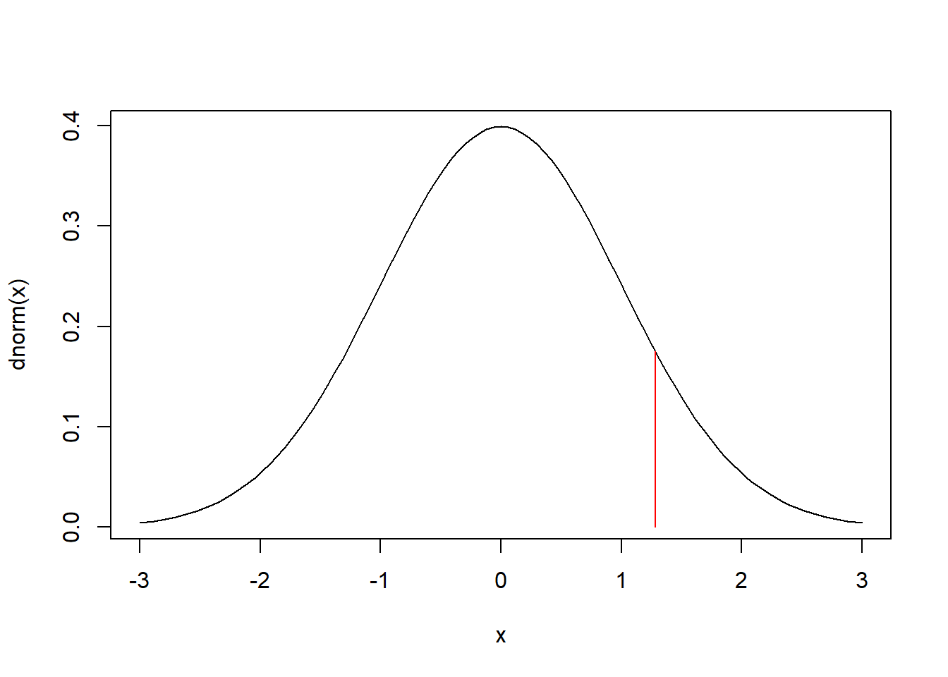
We can plot the standard Normal probability density function and mark the 90th percentile using:
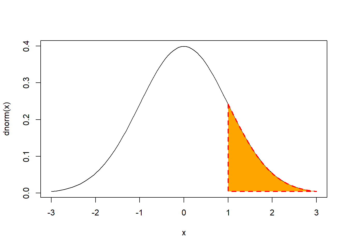
We can shade the area under the N(0,1) probability desnity function to the right of the 90th percentile using:
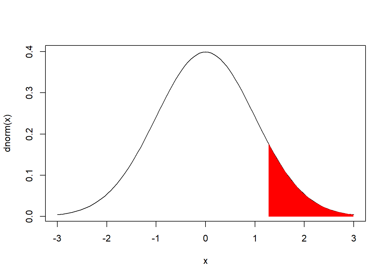
Or:
curve(dnorm,-3,3)
polygon(c(rep(1,201),rev(seq(1,3,.01))),c(dnorm(seq(1,3,.01)),
dnorm(rev(seq(1,3,.01)))), col = "orange", lty = 2, lwd = 2, border = "red")